 Photo by Tisma Jrdl on Unsplash
In the previous post, we looked at T-tests to compare the means of one or two samples. The T-tests can still be used for more than two samples but there are two issues with it :
- It will be tedious to compare every sample with every other samples
- The probability of making Type I error -False Positive (when we reject Null instead of failing to reject) multiples exponentially.
The ANOVA methods were developed by Ronald Fisher as an extension for t and z tests. They measure the between-group variability vs the within-group variability. They can be used to compare two or more groups and find if there is a relationship that exists between them.
There are 2 types of ANOVA tests
- One-way ANOVA is used when there is one independent variable (with more than factor 2 levels) and one dependent variable
- Two-way ANOVA is used when there are more one independent variable (with more than factor 2 levels each) and one dependent variable
One-way ANOVA
- The ANOVA is different from other tests as we have to compute different measures and then use them to calculate the F-score.
- The measures that need to be computed for updating the table are given below
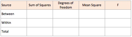
- Total Sum of Squares \(SS_{T}\) is the sum of the difference between each value y from the grand mean for N observations \(SS_{T} = \sum (y - \bar{y}^2) = \sum y^2 - \frac{(\sum y)^2}{N}\)
- Sum of Squares Between \(SS_{B}\) for k groups, \(n_{k}\) observations in group k and \(\bar y_{k}\) being the mean of the group k is given by \(SS_{B} = \sum n_{k} (\bar y_{k} - \bar {y})^2\)
- Sum of Squares Within groups \(SS_{W} = SS_{T} - SS_{B}\)
- The degrees of freedom are given by
- \(df_{Total} = N - 1\)
- \(df_{Between} = k - 1\)
- \(df_{Within} = N - k\)
- We then calculate the mean square error with the associated degrees of freedom.
- \(MS_{B} = \frac {SS_{B}}{df_{Between}}\) measures between-group variability
- \(MS_{W} = \frac {SS_{W}}{df_{Within}}\) measures variability within each of the groups
- And finally the F statistic is the ratio \(\frac {MS_{B}}{MS_{W}}\)
- When the null hypothesis is true any difference among the sample means are only due to chance and MSB and MSW should be equal
- F will be larger when \(MS_{B}\) will be larger than \(MS_{W}\), indicate a strong evidence against the null hypothesis. If there is no difference between the groups it will be close to 1 (accept null hypothesis)
Two way ANOVA
- In one-way ANOVA, we had one dependent variable and one independent variable.
- In two way ANOVA we can have more than one independent variables, so we need to calculate a ratio that measures not only the variation between the dependent and independent variables, but also the interaction between the two independent variables.
Post-hoc analysis
- The ANOVA test gives us the significant variables for which the group means are different but if we have to know which pairs of the groups are different then we need to run post-hoc analysis
- Couple of methods of post-hoc analysis are Tukey Honest Significant Differences and Bonerroni post-hoc analysis
Example
- We will use the ToothGrowth dataset in R.
- The dataset has the observations of the tooth growth in 60 guinea pigs which were administered three doses of Vitamin C (0.1, 1 and 2 mg/day).
- It also has two supplement types using which these doses were administered – OJ (Orange Juice) and VC (ascorbic acid which is a form Vitamin C)
- A quick look at the boxplot indicates there are couple of outliers but we will ignore them. It also indicates that Dose 2 resulted in longer tooth growth and so also Dose 1 given in Orange Juice
str(ToothGrowth)## 'data.frame': 60 obs. of 3 variables:
## $ len : num 4.2 11.5 7.3 5.8 6.4 10 11.2 11.2 5.2 7 ...
## $ supp: Factor w/ 2 levels "OJ","VC": 2 2 2 2 2 2 2 2 2 2 ...
## $ dose: num 0.5 0.5 0.5 0.5 0.5 0.5 0.5 0.5 0.5 0.5 ...ToothGrowth$dose <- as.factor(ToothGrowth$dose)
ggplot(data=ToothGrowth) +
geom_boxplot(aes(x=dose,y=len,fill=supp)) +
labs(subtitle="Box plot of tooth growth for various doses"
,caption = varPlotCaption) +
theme_darklightmix(color_theme = ggplot_color_theme) +
scale_fill_brewer(palette = "Set3")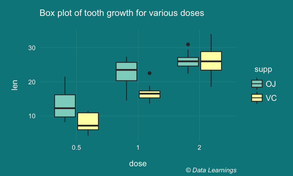
We will run one-way ANOVA on dosage and supplement separately and then run the two-way ANOVA with both of them together with their interaction
One-way ANOVA on dose
- Null hypothesis :
- Mean tooth growth for the 3 doses is same
- Intepretation of the results
- p-value < 0.001 :
- Reject the null hypothesis i.e
- Mean tooth growth is not the same ie different doses have different effect on the tooth growth
- F Statistic of 105 :
- Much higher than the critical value of 12.01 at p=0.05
- ie between group variability (MSB) is much higher than within group variability (MSW)
- TukeyHSD :
- Mean tooth growth is higher for larger doses
- p-value < 0.001 :
summary(aov(len~dose,data=ToothGrowth))## Df Sum Sq Mean Sq F value Pr(>F)
## dose 2 2426 1213 67.42 0.000000000000000953 ***
## Residuals 57 1026 18
## ---
## Signif. codes: 0 '***' 0.001 '**' 0.01 '*' 0.05 '.' 0.1 ' ' 1paste("Critical value of F Statisic:",qf(df1=1,df2 = 58, p= 0.05,lower.tail=F))## [1] "Critical value of F Statisic: 4.00687288633273"TukeyHSD(aov(len~factor(dose),data=ToothGrowth))## Tukey multiple comparisons of means
## 95% family-wise confidence level
##
## Fit: aov(formula = len ~ factor(dose), data = ToothGrowth)
##
## $`factor(dose)`
## diff lwr upr p adj
## 1-0.5 9.130 5.901805 12.358195 0.0000000
## 2-0.5 15.495 12.266805 18.723195 0.0000000
## 2-1 6.365 3.136805 9.593195 0.0000425One-way ANOVA on supplement type
- Null hypothesis :
- Mean tooth growth for the 2 supplement types is same
- Interpretation of results
- p-value > 0.05 :
- Accept the null hypothesis i.e
- Mean tooth growth is the same ie different supplement types have no effect on the tooth growth
- F Statistic of 3.668 :
- Lower than the critical value of 4 at p=0.05
- ie between group variability (MSB) is slightly higher than within group variability (MSW)
- TukeyHSD :
- No TukeyHSD as the null hypothesis is not rejected and hence no need to quantify the effects
- p-value > 0.05 :
summary(aov(len~supp,data=ToothGrowth))## Df Sum Sq Mean Sq F value Pr(>F)
## supp 1 205 205.35 3.668 0.0604 .
## Residuals 58 3247 55.98
## ---
## Signif. codes: 0 '***' 0.001 '**' 0.01 '*' 0.05 '.' 0.1 ' ' 1paste("Critical value of F Statisic:",qf(df1=1,df2 = 58, p= 0.05,lower.tail=F))## [1] "Critical value of F Statisic: 4.00687288633273"Two-way ANOVA on both
- Null hypothesis :
- Mean tooth growth for the 3 doses is same
- Mean tooth growth for the 2 supplement types is same
- The interaction between the dose and supplement type has no effect on the tooth growth
- Interpretation of results
- p-values :
- Dose has p-value < 0.05
- Reject the null hypothesis that the 3 doses have the same effect on tooth growth ie
- The 3 doses are significantly different as seen in the One-Way ANOVA
- Supplement type now has p-value < 0.05
- Reject the null hypothesis that the 2 supplement types have same effect on tooth growth ie
- The supp type now has significant effect on the tooth growth, after controling for the level of dose and the interaction effect dose * supp
- dose:supp has p-value < 0.05
- Reject the null hypothesis
- If the significant value was chosen at say 0.02 then we could have accepted the null hypothesis ie the interaction has no effect on tooth growth
- Dose has p-value < 0.05
- TukeyHSD :
- dose
- The interpretaton for dose is same as that in One-way ANOVA
- supp :
- The mean tooth growth of VC is lower than that achieved by OJ (diff of -3.7)
- Even though in this case the Tukey HSD is not needed as there are only two factor levels
- dose*supp :
- We will look at couple of cases
- 0.5:VC-2:OJ : The mean tooth growth due to 0.5:VC is much lower than 2:OJ and the effect is significant with p-adj < 0.05
- 2:VC-1:OJ : The diff in mean tooth growth is 3.44 with a p adj of > 0.05 indicating that they have the same/similar effect on tooth growth
- dose
- p-values :
summary(aov(len~dose*supp,data=ToothGrowth))## Df Sum Sq Mean Sq F value Pr(>F)
## dose 2 2426.4 1213.2 92.000 < 0.0000000000000002 ***
## supp 1 205.4 205.4 15.572 0.000231 ***
## dose:supp 2 108.3 54.2 4.107 0.021860 *
## Residuals 54 712.1 13.2
## ---
## Signif. codes: 0 '***' 0.001 '**' 0.01 '*' 0.05 '.' 0.1 ' ' 1#paste("Critical value of F Statisic:",qf(df1=1,df2 = 58, p= 0.05,lower.tail=F))
TukeyHSD(aov(len~factor(dose)*supp,data=ToothGrowth))## Tukey multiple comparisons of means
## 95% family-wise confidence level
##
## Fit: aov(formula = len ~ factor(dose) * supp, data = ToothGrowth)
##
## $`factor(dose)`
## diff lwr upr p adj
## 1-0.5 9.130 6.362488 11.897512 0.0000000
## 2-0.5 15.495 12.727488 18.262512 0.0000000
## 2-1 6.365 3.597488 9.132512 0.0000027
##
## $supp
## diff lwr upr p adj
## VC-OJ -3.7 -5.579828 -1.820172 0.0002312
##
## $`factor(dose):supp`
## diff lwr upr p adj
## 1:OJ-0.5:OJ 9.47 4.671876 14.2681238 0.0000046
## 2:OJ-0.5:OJ 12.83 8.031876 17.6281238 0.0000000
## 0.5:VC-0.5:OJ -5.25 -10.048124 -0.4518762 0.0242521
## 1:VC-0.5:OJ 3.54 -1.258124 8.3381238 0.2640208
## 2:VC-0.5:OJ 12.91 8.111876 17.7081238 0.0000000
## 2:OJ-1:OJ 3.36 -1.438124 8.1581238 0.3187361
## 0.5:VC-1:OJ -14.72 -19.518124 -9.9218762 0.0000000
## 1:VC-1:OJ -5.93 -10.728124 -1.1318762 0.0073930
## 2:VC-1:OJ 3.44 -1.358124 8.2381238 0.2936430
## 0.5:VC-2:OJ -18.08 -22.878124 -13.2818762 0.0000000
## 1:VC-2:OJ -9.29 -14.088124 -4.4918762 0.0000069
## 2:VC-2:OJ 0.08 -4.718124 4.8781238 1.0000000
## 1:VC-0.5:VC 8.79 3.991876 13.5881238 0.0000210
## 2:VC-0.5:VC 18.16 13.361876 22.9581238 0.0000000
## 2:VC-1:VC 9.37 4.571876 14.1681238 0.0000058Inference
- dose has the most significant effect on tooth growth
- supplement type on its own doesn’t have much effect but its effect increases when combined with the dose variable
- Thus changing supplement methods or the dose of vitamin C, will significantly impact the tooth growth
ANOVA Assumptions
- ANOVA has three assumptions
- All observations are independent of one another and randomly selected from the population which they represent
- The variance across groups must be almost the same(homoscedasticity)
- The distribution should be approximately normal at each factor level
The homogeneity of the variances can be verified using the residuals vs fitted plot which shows that the residuals are uniformly distributed around the x axis and that there is no relationship between residuals and fitted values. It can also be checked using car::leveneTest()
plot(aov(len~dose*supp,data=ToothGrowth),1)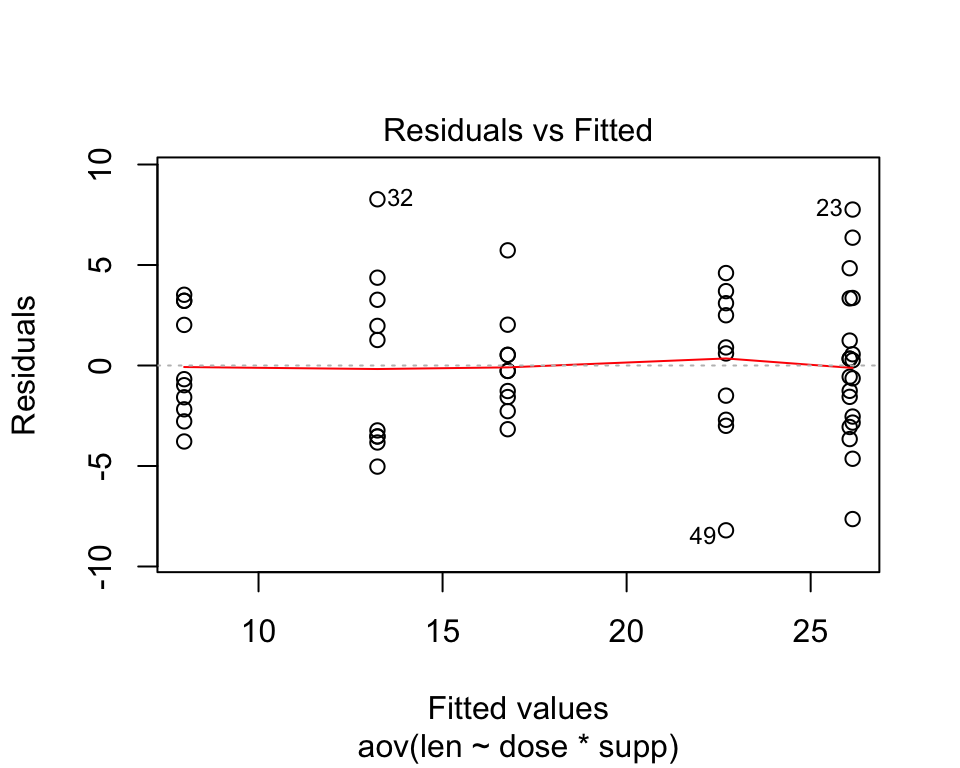
The normality assumption can be checked using the QQ plot which shows that the residuals are along the diagonal line It can also be verified using the Shapiro Wilk test. If it failed, then we would do transformation of the dependent variable.
plot(aov(len~dose*supp,data=ToothGrowth),2)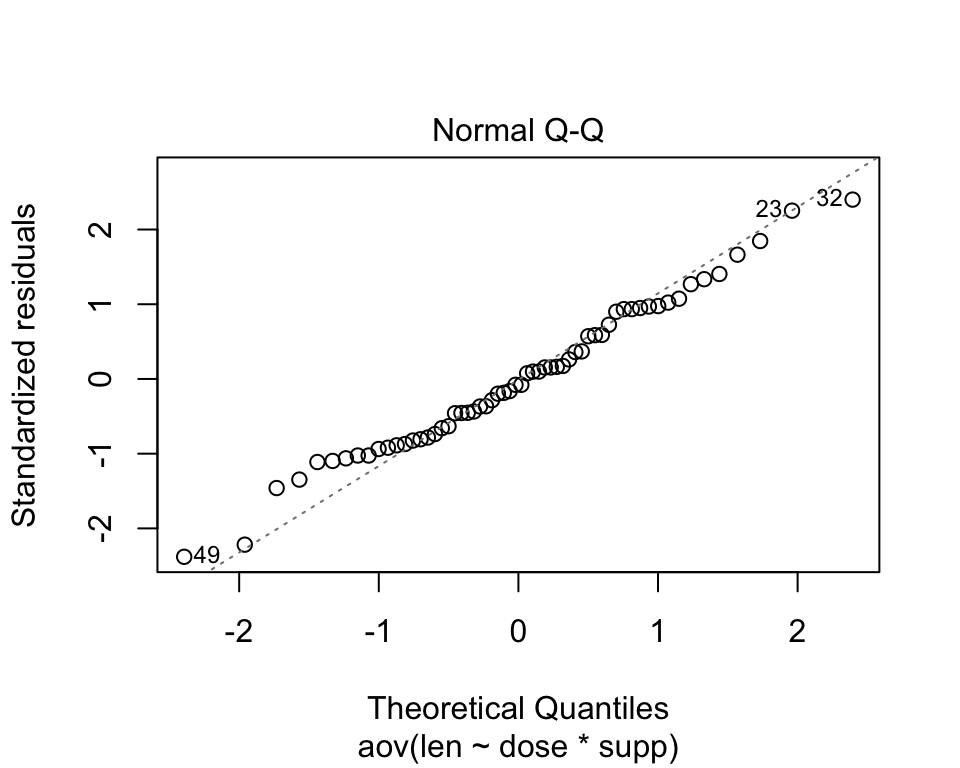
shapiro.test(x = residuals(aov(len~dose*supp,data=ToothGrowth)))##
## Shapiro-Wilk normality test
##
## data: residuals(aov(len ~ dose * supp, data = ToothGrowth))
## W = 0.98499, p-value = 0.6694Unbalanced ANOVA
- The ToothGrowth dataset was balanced the number of observations in each group were equal
- If it was not balanced then we would use car::Anova()
table(ToothGrowth$supp,ToothGrowth$dose) %>%
kable(format.args = list(decimal.mark = '.', big.mark = ",")) %>%
kable_styling(bootstrap_options = "condensed"
            ,full_width = FALSE
            ,position = "center"
,font_size = 10)| 0.5 | 1 | 2 | |
|---|---|---|---|
| OJ | 10 | 10 | 10 |
| VC | 10 | 10 | 10 |
Summary
- The null hypothesis for ANOVA is that the mean of the dependent variable is the same for all groups
- Further learning
- Unbalanced design experiments for ANOVA
- Three classes of models
- Fixed-effects model (class I)
- Random-effects model (class II)
- Mixed-effects model (class III)
- See also http://www.sthda.com/english/wiki/two-way-anova-test-in-r