ASGS Background

The Australian Bureau of Statistics publishes the Australian Statistical Geography Standard (ASGS). These consists of geospatial data that can be used for plotting the geographical boundaries and also integrated with other statistical data. The framework

At the lowest level there is the NAMF. It is the framework is used for verification and management of physically addresses with the aim of one address = one location. Rest of the levels are shown below Source:

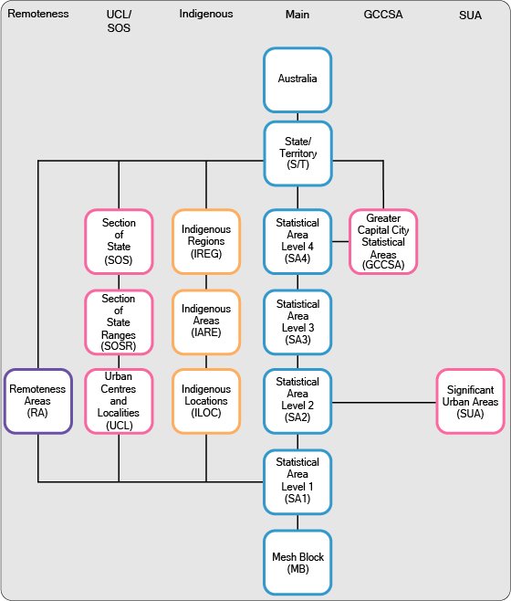
• The next level is the ASGS Mesh blocks.
  • They are the smallest geographical areas and form the basis for the larger higher level regions.
  • The 2016 ASGS contains 358,122 Mesh blocks covering the whole of Australia.
  • Each Mesh Block is uniquely identified by a 11 digit id consisting of State and Territory identifier (1 digit) and a Mesh block identifier (10 digits).
• On top of the Mesh Block, there are four statistical area levels as shown below.
  • SA1 has a population ranging from 200-800 and are the aggregation of the Mesh Blocks
  • SA2 has between 3000-25000 persons and consider the suburb and locality boundaries
  • SA3 has population of 20000+ and consist of regional towns, cities and suburbs around major urban areas
  • SA4 have population of 100000+

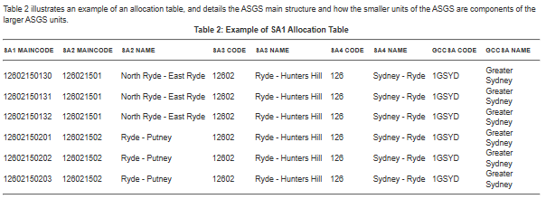
• ABS releases different statistics at each of these level. For example the Labour Force Survey data is released at SA3 level. Although, most of statistics are released at SA2 level.

• Correspondences
  • Indexes that can be used for mapping one statistical area to another.
  • These can be downloaded from here
• The Geospatial data is provided in three formats :
  • ESRI Shapefiles : The shapefile format is a geospatial vector data format for geographic information system software. It is developed and regulated by Esri as a mostly open specification for data interoperability among Esri and other GIS software products
  • MapInfo Tab format : The MapInfo TAB format is a geospatial vector data format for geographic information systems software
  • MapInfo Interchange format : MapInfo Interchange Format is a map and database exporting file format of MapInfo software product

• Note on Raster and Vector graphics : Raster graphics like .bmp,.jpg, .tif, .gif are made up of pixels, they occupy more space. Vector graphics like .svg .eps, .pdf, are composed of mathematical paths and result in smaller file sizes

Shapefiles

I will use the ESRI shapefiles for this post. The ESRI Shapefiles are available this location.

• A shapefile is an Esri vector data storage format for storing the location, shape, and attributes of geographic features
• Shapefiles are a simple, nontopological format for storing the geometric location and attribute information of geographic features. A shapefile is one of the spatial data formats that you can work with and edit in ArcGIS.
• The shapefile format defines the geometry and attributes of geographically referenced features in three or more files with specific file extensions that should be stored in the same project workspace. They are:
  • shp—The main file that stores the feature geometry; required.
  • shx—The index file that stores the index of the feature geometry; required.
  • dbf—The dBASE table that stores the attribute information of features; required.
  • .prj—The file that stores the coordinate system information; used by ArcGIS.

I have downloaded the SA2 level shape file

R Packages

R has several packages for working with spatial data. The best resource is the Spatial Cran task view. In this post, I will use these packages

• Data Manipulation
  • sp : Older package and supposedly slower. sp objects can be created using rgdal::readOGR function. Internally called by some other packages.
  • rgdal : This package is used for translating raster and vector geospatial data formats. It is based on the gdal project which supports several vector and raster drivers. Depends on sp
  • rgeos : Depends on sp
  • sf (simple features) is newer package for working with spatial data in R. sf functions start with st
• Data visualisation
  • base R
  • leaflet
  • tmap
  • ggmap

Data Loading

First, I will use the readOGR function from the rgdal package to load the ESRI shapefiles.

The readOGR function is used for reading a OGR data source. Since we are reading a shapefile, the layer argument will have the the filename without the .shp extension. The function has returned the object of class “SpatialPolygonsDataFrame”.

In R, the objects S4 class can be accessed using the @ operator (vs the $ operator used for accessing S3 class objects). The @data slot gives the non-geographic attribute data and the @polygons slot gives the geometric paths for constructing the spatial objects. We can pass the object to the plot function

obj_rgdal <- rgdal::readOGR(dsn=here::here('content','post','data','2020-05-01-geographic-data-and-visualisation-in-r',
                                           'ESRI-Shape-files-1270055001_sa2_2016_aust_shape'),layer="SA2_2016_AUST" )

## OGR data source with driver: ESRI Shapefile 
## Source: "/Mac Backup/OneDrive/R/Blogs/datablog/content/post/data/2020-05-01-geographic-data-and-visualisation-in-r/ESRI-Shape-files-1270055001_sa2_2016_aust_shape", layer: "SA2_2016_AUST"
## with 2310 features
## It has 12 fields

class(obj_rgdal)

## [1] "SpatialPolygonsDataFrame"
## attr(,"package")
## [1] "sp"

# Commented as it is not responsive on a Mobile
# head(obj_rgdal@data) %>%
# kable(format.args = list(decimal.mark = '.', big.mark = ",")) %>%
# kable_styling(bootstrap_options = "condensed"
#             ,full_width = FALSE
#             ,position = "left"
#             ,font_size = 10)

Alternatively, data can also be loaded using the st_read function in the sf package.

sf objects are just data-frames that are collections of spatial objects. Each row is a spatial object (e.g. a polygon), that may have data associated with it (e.g. its area) and a special geo variable that contains the coordinates.

The readOGR function drops NULL geometries, I will do the same for the obj_sf so that the visualisations in the next sections are consistent.

obj_sf <- sf::st_read(dsn=here::here('content','post','data','2020-05-01-geographic-data-and-visualisation-in-r',
                                           'ESRI-Shape-files-1270055001_sa2_2016_aust_shape'),layer="SA2_2016_AUST")

## Reading layer `SA2_2016_AUST' from data source `/Mac Backup/OneDrive/R/Blogs/datablog/content/post/data/2020-05-01-geographic-data-and-visualisation-in-r/ESRI-Shape-files-1270055001_sa2_2016_aust_shape' using driver `ESRI Shapefile'
## Simple feature collection with 2310 features and 12 fields (with 18 geometries empty)
## geometry type:  MULTIPOLYGON
## dimension:      XY
## bbox:           xmin: 96.81694 ymin: -43.74051 xmax: 167.998 ymax: -9.142176
## CRS:            4283

class(obj_sf)

## [1] "sf"         "data.frame"

#head(obj_sf[,which(!names(obj_sf) == "geometry")],10)  


#Drop null geometries
obj_sf <- obj_sf[!st_is_empty(obj_sf),]

Distance from Brisbane City Centre

One of the common task in the spatial data is to find areas within certain distance. Here, I use the rgeos::gCentroid function to get the centroids for each of the suburbs. And then the sp::spDistsN1 function to get the distance of these centroids from the Brisbane city with long/lat of (153.0231,-27.468326)

I have not looked into the details, but it seems like the function calculates using Euclidean distance. This assumes the earth is flat. But as the Earth is spherical what we need is to calculate the GCD (Greater Circle Distance). At some point I will look at the great circle funtions in this article.

SA2_centroids <- rgeos::gCentroid(obj_rgdal, byid = TRUE,id = obj_rgdal@data$SA2_NAME16)
brisbane_city <- c(153.0231,-27.468326)
kms_city_center <- round(sp::spDistsN1(as.matrix(data.frame(SA2_centroids)[,c("x","y")]),brisbane_city,longlat = TRUE),2)

#confirm all suburbs are included
length(kms_city_center)

## [1] 2292

# #The same can also be acheived using sf package but I need to fix this error
# geoms <- st_geometry(obj_sf)
# SA2_centroids <- do.call(rbind, st_centroid(geoms))
# class(SA2_centroids)
# colnames(SA2_centroids) <- c("x","y")
# head(SA2_centroids)
# kms_city_center2 <- round(sp::spDistsN1(SA2_centroids,brisbane_city,longlat = TRUE),2)

Data Visualisation

plot(obj_rgdal[kms_city_center < 10,], main="Suburbs within 10 kms - rgdal object")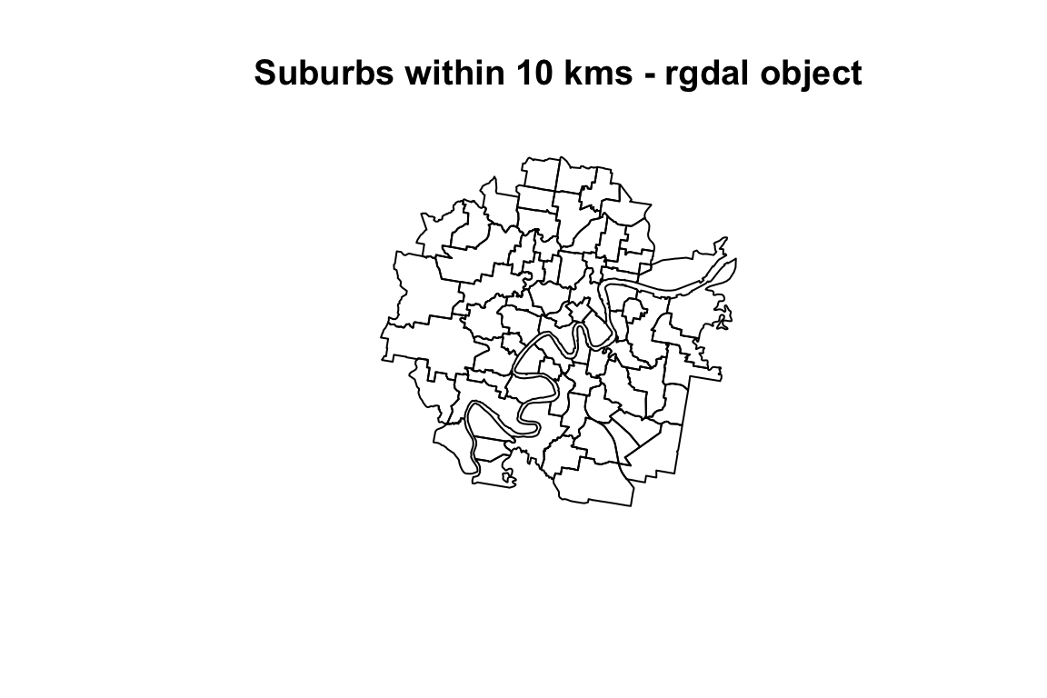

plot(obj_sf[kms_city_center < 10,"geometry"],main = "Suburbs within 10 kms - sf object")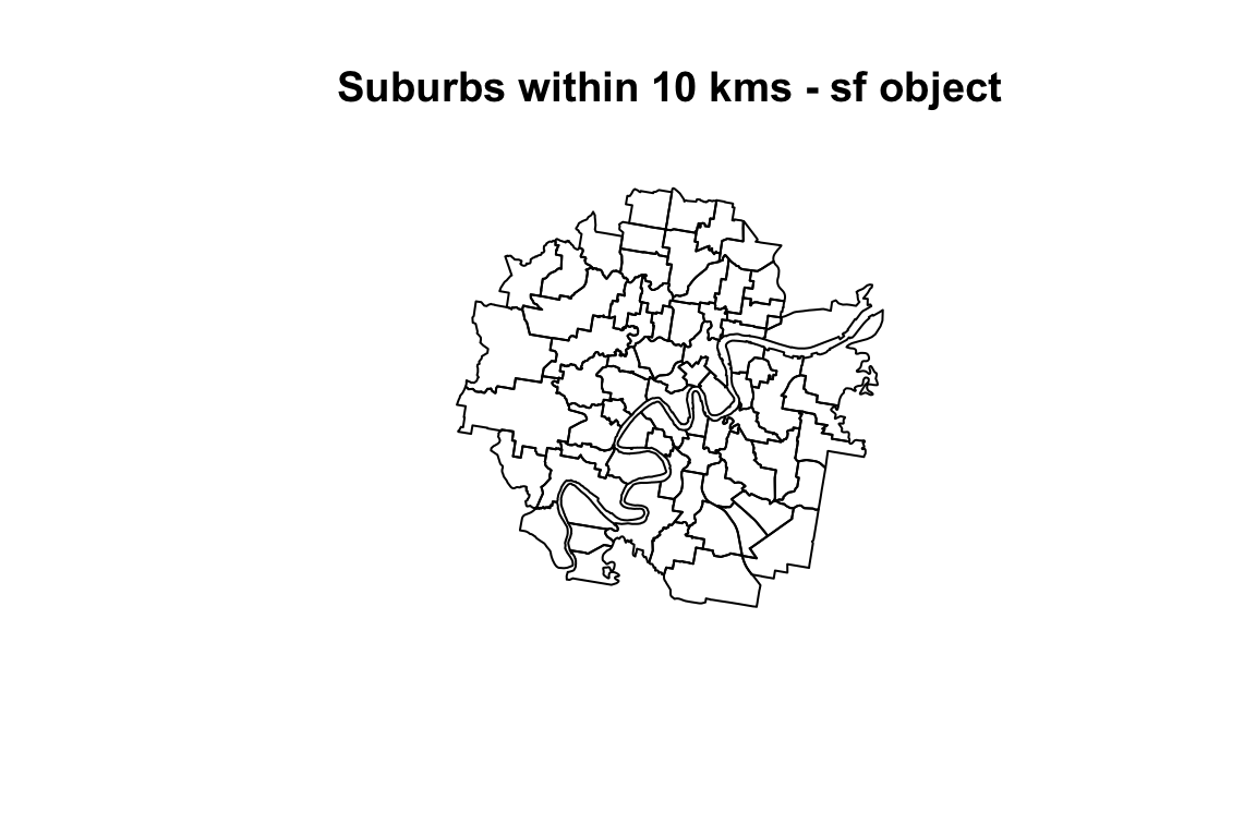

Using Leaflet

• Leaflet is a open source Javascript library
• It is interactive and hence can be used in webapps developed using Shiny

# leaflet(obj_rgdal[kms_city_center < 10,]) %>% 
#   addTiles() %>%
#   addPolylines(stroke = TRUE, weight = 1,color = "blue") 

leaflet(obj_sf[kms_city_center < 10,]) %>% 
  addTiles() %>%
  addPolylines(stroke = TRUE, weight = 1,color = "blue") 

Using tmap

• Based on the principles of Grammer of graphics, tmap is a thematic maps package
• Similar to ggplot, can create facets, easier to customize
• Personally, I feel the plots tmap plots look beautiful
• Can be made interactive using tmap_mode("view")
• Resource

#Simple quick map
#tmap::qtm(obj_sf[kms_city_center < 10,])

#Add the population stored in the Tot_P_P to the obj_sf
populationQLD <- read.csv(here::here('content','post','data','2020-05-01-geographic-data-and-visualisation-in-r',
                                           '2016Census_G01_QLD_SA2.csv'))
# head(obj_sf)
# head(populationQLD[,c("SA2_MAINCODE_2016","Tot_P_P")])

obj_sf <- merge(obj_sf,populationQLD[,c("SA2_MAINCODE_2016","Tot_P_P")]
                ,all.x = T
                ,by.x = "SA2_MAIN16"
                ,by.y = "SA2_MAINCODE_2016")

#tmap_mode("view")
#tm_view(text.size.variable = TRUE)

tm_shape(obj_sf[kms_city_center < 20,]) +
  tm_polygons("Tot_P_P") +
  tm_text("SA2_NAME16",size="AREA")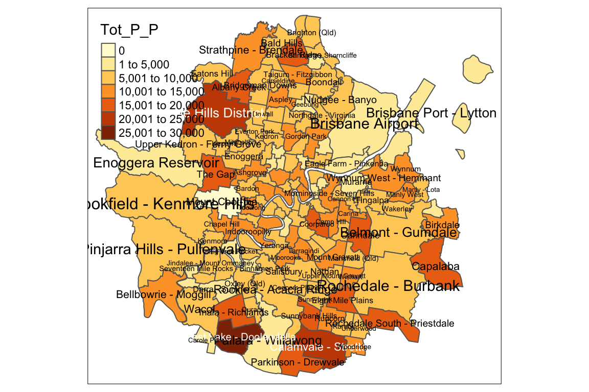

Using ggmap

A collection of functions to visualize spatial data and models on top of static maps from various online sources (e.g Google Maps and Stamen Maps). It includes tools common to those tasks, including functions for geolocation and routing.

obj_sf[kms_city_center < 10,] %>%
  ggplot() +
  geom_sf(aes(fill = AREASQKM16)) +
    scale_fill_viridis_c(trans = "sqrt", alpha = .4)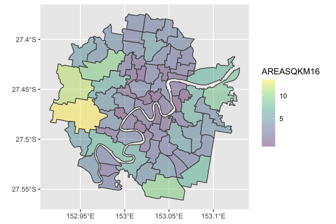

Summary

This was a quick post for getting started with geospatial data in R. I will continue to update it as and when I work on more use cases.

• The Australian ASGS data is available at different levels : Mesh Blocks, SA1, SA2 and so on
• ESRI shapefiles are one of the formats used in geospatial data
• There are several R packages for data manipulation :
  • sp,rgdal and rgeos are the older packages
  • sf is a newer package
• Visualisation can be done using
  • Base R
  • leaflet
  • tmap
  • ggmap
  • and many others
• References/Resources
  • CRAN Task View
  • Visualising Spatial data in R
  • sp or sf
  • leaflet
  • tmap
  • ggmap