 Photo by Tom Wheatley on Unsplash
In the previous post, we looked at some of the basic statistical concepts. In this post, we will look at how t-tests can be used to making inferences about the population. We will use the iris dataset.
T-test vs Z-Test
- T-tests are used when the sample size is below 30 and when we don’t know the population standard deviation. If we know the population standard deviation and the sample size is above 30 then we use the Z-Test and its associated z-score
- T-tests are important because usually we don’t know anything about the population and we have to rely on the samples to make inferences about the population
T-tests
- Also known as Student’s T Test are tests used for comparing means and how different they are from each other and whether those differences are only due to chance. They can be used to find if two sets of data are significantly different from each other.
- The T-tests gives us the t-score
- The t score is a ratio between the difference between two groups and the difference within the groups
- It tells us whether one group is statistically significant to the other group
- A large t-score tells us that the groups are different. A small t-score tells us that the groups are similar
- A t score of 3 means that the groups are three times as different from each other as they are within each other.
- It is analogous to signal-to-noise ratio as explained in the One sample t-test section
- There are 3 types of T tests
- One sample t-test : Compare the mean of a population with a theoretical value
- Unpaired or Independent Two sample t-test : Compare the mean of two independent samples
- Paired or Dependent Two sample t-test : Compare the means between two related groups of samples
One Sample t-test
- The formula for 1-Sample t test is \(t = \frac{\overline{X} - \mu_{0} } { \sigma / \sqrt{n}}\)
- \(\overline{X}\) is the mean of the sample
- \(\mu_{0}\) is the null hypothesis value
- \(\sigma\) is the standard deviation
- \(\sqrt{n}\) is the square root of the sample size
- The equation is similar to the signal-to-noise ratio.
- The numerator is simply the difference between the mean of the sample and the expected value of the mean (of the population).
- The null hypothesis is that sample has been taken from the population. This will happen when both the values are same and the equation gives 0 and the null hypotheses gets accepted.
- As the difference increases (either +ve or -ve), the signal also increases, possibly leading to the rejection of the null hypothesis.
- The denominator in the formula is actually the standard error of the mean, which is a measure of variability in the sample.
- It measures the accuracy with which a sample represents a population.
- In statistics, a sample mean deviates from the actual mean of a population; this deviation is the standard error.
- A higher number indicates that the sample estimate is less accurate as it has more random error.
- This random error is the noise.
- If the noise is high, its possible that the numerator gets a large value but that doesn’t mean the null hypotheses can be rejected. Thats why we can use the t-test to see if the signal stands out from the noise or its a random error in the sample
- For example a t-value of 10 implies the signal is 10 times the noise and probably a sign that the null hypothesis can be rejected and the alternate hypothesis that the sample is different from the population can be accepted.
- A t-value of 0 indicates that the sample results exactly equal the null hypothesis.
Example 1
Lets use the Sepal.Width to illustrate the concept
p1 <- iris %>%
  ggplot(aes(x=Sepal.Width)) +
  geom_histogram(fill="cornsilk",binwidth=0.2) +
  labs(x="Sepal Width"
       ,y="Count"
       ,subtitle="Approx normal distribution of Sepal Width"
    #   ,caption = varPlotCaption
    ) +
  theme_darklightmix(color_theme = ggplot_color_theme) +
  scale_fill_brewer(palette = "Set3")

p2 <- iris %>%
  ggplot(aes(y=Sepal.Width)) +
  geom_boxplot(fill="cornsilk"
               ) +
  labs(x=""
       ,y="Sepal Width"
       ,subtitle="Sepal Width boxplot"
     #  ,caption = varPlotCaption
     ) +
  theme_darklightmix(color_theme = ggplot_color_theme) +
  scale_fill_brewer(palette = "Set3")

grid.arrange(p1, p2, ncol=2)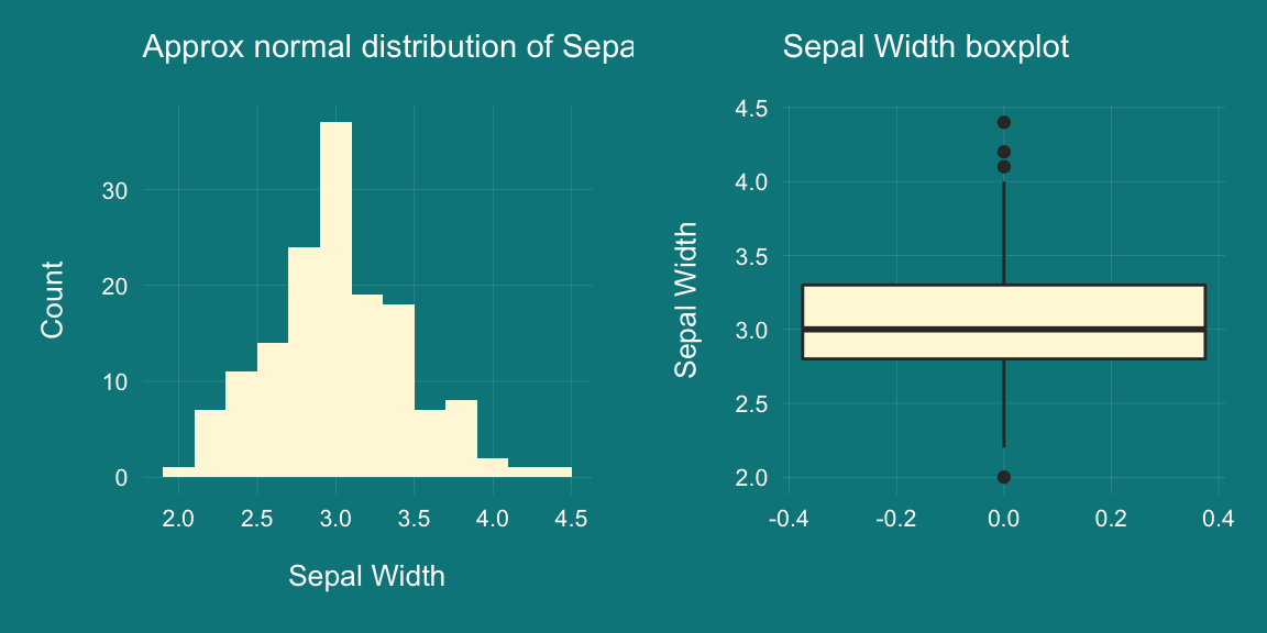
- We will take sample of 10 observations and hypothecate that this sample belong to the population and its mean is equal to the mean of the population (ie 3.057333).
- We get low t-score of 0.62714 and high p-value of 0.5361 proving our hypothesis. If the p-value was <0.05 we would have rejected the null hpypothesis
set.seed(2)
t.test(sample(iris$Sepal.Width,10),
 mu=mean(iris$Sepal.Width))
##
## One Sample t-test
##
## data: sample(iris$Sepal.Width, 10)
## t = 1.158, df = 9, p-value = 0.2767
## alternative hypothesis: true mean is not equal to 3.057333
## 95 percent confidence interval:
## 2.902223 3.537777
## sample estimates:
## mean of x
## 3.22Example 2
- Lets formulate another hypothesis and state that the Sepal.Width sample is drawn from the Petal.Width population.
- We can see that the t-score is very high 12.5 and the p-value for the test is very low. Thus disproving our hypothesis as expected.
set.seed(2)
t.test(sample(iris$Sepal.Width,10), mu=mean(iris$Petal.Width))
##
## One Sample t-test
##
## data: sample(iris$Sepal.Width, 10)
## t = 14.384, df = 9, p-value = 1.622e-07
## alternative hypothesis: true mean is not equal to 1.199333
## 95 percent confidence interval:
## 2.902223 3.537777
## sample estimates:
## mean of x
## 3.22Unpaired or Independent Two Sample t-test
- Two sample tests are used to determine how different two samples are.
- The assumption are that both the samples are independent of each other and they follow normal distribution.
- The formula for Unpaired two sample T-test is given by \(t =\frac{(\overline{X_{1}} - \overline{X_{2}}) - (\mu_{1} - \mu_{2})}{SE _{(\overline{X_{1}} - \overline{X_{2}})}}\)
- \(SE _{(\overline{X_{1}} - \overline{X_{2}})} = \sqrt{\frac{\sigma_{1}^2}{n_{1}} + \frac{\sigma_{2}^2}{n_{2}}}\)
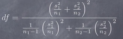
- The formula to calculate the degrees of freedom is given below. This will be used for finding the p-value for the above t-value
Example 1 : Two groups from same population
- Lets randomly take 2 sets of 20 values from Sepal width (group 1 and group 2).
- The null hypothesis is both groups belong to the same population. We get a low tscore of 1.32 and a high probability of 19% in favour of the null hypotheses
set.seed(123)
t.test(sample(iris$Sepal.Width,20),sample(iris$Sepal.Width,20))
##
## Welch Two Sample t-test
##
## data: sample(iris$Sepal.Width, 20) and sample(iris$Sepal.Width, 20)
## t = -0.50549, df = 34.315, p-value = 0.6164
## alternative hypothesis: true difference in means is not equal to 0
## 95 percent confidence interval:
## -0.3513272 0.2113272
## sample estimates:
## mean of x mean of y
## 2.955 3.025- Given the t-value and the degrees of freedom, the p-value can be calculated as follows
2*pt(q=-abs(1.3238),df=30.731)## [1] 0.195333Example 2 : Two groups from different population
- Lets randomly take 2 sets of 20 values from Sepal width (group 1) and from Petal Width (group 2).
- The null hypothesis is both groups belong to the same population.
- We get a high t-score of 8.84 and a very low probability in favour of the null hypotheses, implying that the null hypothesis can be rejected
set.seed(123)
t.test(sample(iris$Sepal.Width,20),sample(iris$Petal.Width,20))
##
## Welch Two Sample t-test
##
## data: sample(iris$Sepal.Width, 20) and sample(iris$Petal.Width, 20)
## t = 9.933, df = 27.922, p-value = 1.15e-10
## alternative hypothesis: true difference in means is not equal to 0
## 95 percent confidence interval:
## 1.416847 2.153153
## sample estimates:
## mean of x mean of y
## 2.955 1.170Note that : “Welch’s t-test is an adaptation of Student’s t-test, that is more reliable when the two samples have unequal variances (variance = square of standard deviation) and unequal sample sizes”
Paired or Dependent Two Sample t-test
- It is essentially same as a one sample t-test and is used to compare the means of two related samples i.e when you have two values (pair of values) for the same samples (for example before and after measurements)
- The formula \(t = \frac{\overline{d} - \mu_{0} } { SE _{\overline{d}}}\)
- \(\overline{d}\) is the mean of the differences between the paired values
- The denominator \(SE _{\overline{d}} = \frac{\sigma_{d}}{\sqrt{n}}\) is its standard error
- \(\mu_{0}\) is the null hypothesis value
- For a example a restaurant wants to determine whether their new menu items were effective. Assuming they would use the same “before” and “after” subjects, we can use a paired t-test to calculate the difference within each before-and-after pair of measurements, find the mean of these changes and determine whether this mean of changes is statistically significant
- The paired t-test works well even if the distribution is not normal provided it is symmetric and unimodal and the difference in the paired values is normal.
- For paired t-test the Null hypothesis states that the population mean of the differences equals the hypothesised mean of the differences
Summary
- p-value gives the probability of accepting the null hypothesis, hence a lower p-value indicates low probability of null hypothesis being true
- Examples of a null hypothesis in t-test would be : groups belong to same population, groups are similar
- t-value gives the magnitude of the difference between the groups
- t-value is inversely proportional to p-value. Higher the t, lower the probability of the null hypothesis being True
- p-value is derived using the distribution of the t-values
- Further reading
- This article has good explanation on the signal-to-noise ratio for 2 sample T-test
- This article and this article has the list of all the statistical tests
- Some examples of paired t-test are given here
- Explains how the p-value is derived from the probability distribution function of the test statistic under consideration (this and this and this )