 Photo by Qingbao Meng on Unsplash
It is not always possible to collect data on the entire population, so we take random samples from the population and then use those samples to make predictions or derive inferences about the population. These techniques are referred as Inferential statistics.
- It differs from Descriptive statistics which is used to describe the population data.
- And it differs from Probability in which we use a known population value (parameter) to make prediction about the likelihood of a particular sample value (statistic)
- Descriptive statistics (like measures of central tendency, measures of spread)
- when applied to populations are called
parametersand - when they are applied to samples are called
statistics
- when applied to populations are called
This post consists of some of the notes that I had taken while studying Inferential Statistics. They are not exhaustive and also not in any specific order or structure.
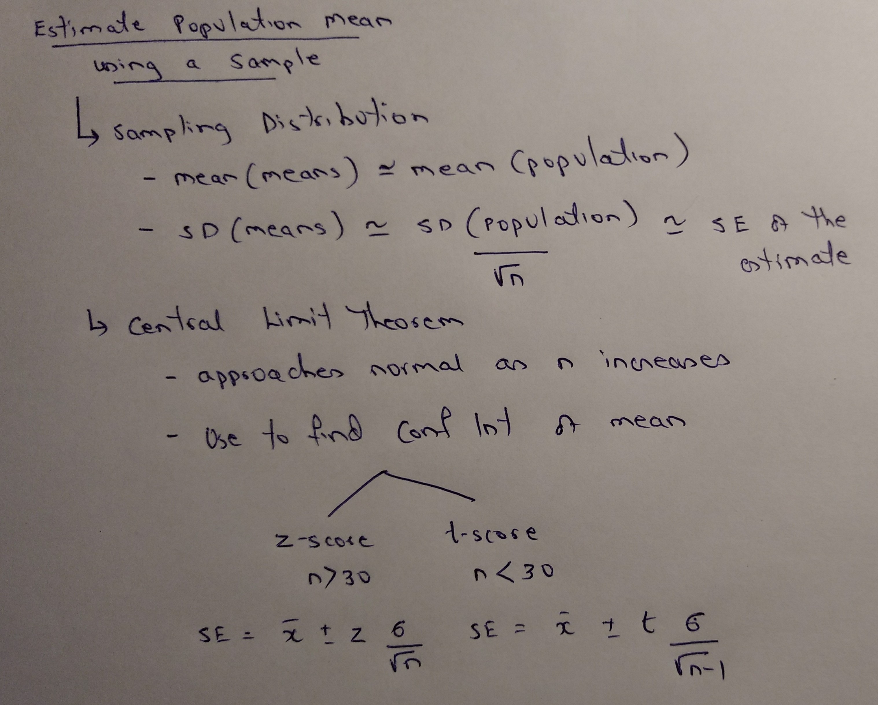
Sampling Distribution
If we take random samples of data from a population, and plot the means of these samples, the resulting distribution that we get is called as the Sampling Distribution
Lets run through an example. We will consider Sepal.Length from the iris dataset as our population. It has mean of 5.8433333 and standard deviation of 0.8280661. And the histogram looks as below
iris %>%
  ggplot(aes(x=Sepal.Length)) +
  geom_histogram(fill="cornsilk",binwidth=0.05) +
  labs(x="Sepal Length"
       ,y="Count"
       ,title="Petals and Sepals"
       ,subtitle="Histogram of Sepal Length"
       ,caption = varPlotCaption) +
  theme_darklightmix(color_theme = ggplot_color_theme) +
  scale_fill_brewer(palette = "Set3")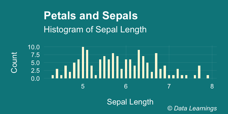
Now, lets take 30 samples (sample size) from this population and repeat it 1000 times. If we plot the means of each of these repeatitions, the resulting distribution that we get is called the Sampling distribution and it is centered around the population mean of 5.84.
If the population size was large, we could have taken larger sample size and done fewer repeats and still we would have got a similar distribution.
set.seed(123)
SL_sample_means <- vector()
for(i in 1 : 1000) {
 SL_sample_means[i] <- mean(sample(iris$Sepal.Length,30))
}


data.frame(Sepal.Length = SL_sample_means) %>%
  ggplot(aes(x=Sepal.Length)) +
  geom_histogram(fill="cornsilk",binwidth=0.05) +
  labs(x="Sepal Length"
       ,y="Count"
       ,title="Petals and Sepals"
       ,subtitle="Histogram of Sepal Length"
       ,caption = varPlotCaption) +
  theme_darklightmix(color_theme = ggplot_color_theme) +
  scale_fill_brewer(palette = "Set3")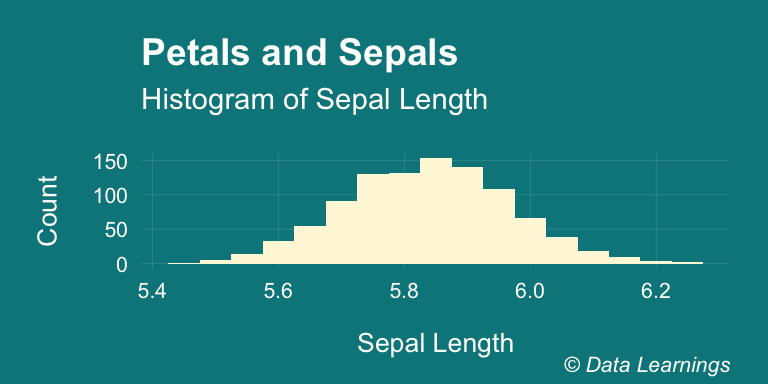
Standard Error
- The variablity of the sample means decreases as sample size increases. The sample means are more tightly clustered around the true mean. This variablity of sample means is called the standard error
s. It is like the standard deviation of a sampling distribution. - In other words, the standard deviation of this sampling distribution approximately equals the SD of the population divided by the square root of the sample size which is the typical error associated with an estimate.
- Thus, the SD of the sample mean given n independent observations from a population with standard deviation \(\sigma\) is given by the formula \(\frac{\sigma } { \sqrt{n}}\).
- The important things to note is that the observations should be independent and a reliable way to do that is to take a random sample consisting of less than 10% of the population.
- The mean and standard deviation are descriptive statistics, whereas the standard error of the mean is descriptive of the random sampling process. i.e the standard error of the sample mean is an estimate of how far the sample mean is likely to be from the population mean, whereas the standard deviation of the sample is the degree to which individuals within the sample differ from the sample mean.
In particular, the standard error of a sample statistic (such as sample mean) is the actual or estimated standard deviation of the error in the process by which it was generated. In other words, it is the actual or estimated standard deviation of the sampling distribution of the sample statistic. The notation for standard error can be any one of SE, SEM (for standard error of measurement or mean), or SE.
If the population standard deviation is finite, the standard error of the mean of the sample will tend to zero with increasing sample size, because the estimate of the population mean will improve, while the standard deviation of the sample will tend to approximate the population standard deviation as the sample size increases.
sd(SL_sample_means)## [1] 0.1298081sd(iris$Sepal.Length)/sqrt(30)## [1] 0.1511835Central Limit Theorem
The Central Limit Theorem states that the distribution of the mean of samples approaches the normal distribution as the sample size n increases. Usually, if the sample size n >= 30 the distribution will be well approximated by the normal distribution, even for skewed populations. Watch out for outliers in the population.
If we can select a single sample of a known size from our population and calculate its mean, we can use the Central Limit Theorem to predict what that true population mean must be within a defined degree of confidence.
The Central Limit Theorem confirms the intuitive notion that as the sample size increases for a random variable, the distribution of the sample means will begin to approximate a normal distribution, with the mean equal to the mean of the underlying population and the standard deviation equal to the standard deviation of the population divided by the square root of the sample size,
n
Confidence interval (CI)
- Confidence interval gives the range of values the particular population parameter will fall between.
- If we know standard deviation of a population then the CI for the mean is given by the formula \(\overline{X} \pm z^{*} \frac {\sigma}{\sqrt{n}}\)
- \(\overline{X}\) is the mean
- \(\sigma\) is the standard deviation of the population
- \(z^{*}\) is the value from the normal distribution
- We can see that \(\frac {\sigma}{\sqrt{n}}\) is the formula for Standard error of the mean
- The \(z^{*}\) values for some confidence intervals are given below
tibble::tribble(
       ~Conf_Int., ~z_Value,
             "80%",     1.28,
             "90%",     1.64,
             "95%",     1.96,
             "98%",     2.33,
             "99%",     2.58
       ) %>%
  kable() %>%
  kable_styling(bootstrap_options = c("striped", "hover"
                                      , "condensed", "responsive")
                ,full_width = F
                ,position = "center"
                #,font_size = 7
)| Conf_Int. | z_Value |
|---|---|
| 80% | 1.28 |
| 90% | 1.64 |
| 95% | 1.96 |
| 98% | 2.33 |
| 99% | 2.58 |
Now, lets find the Confidence interval of the Sample mean. So for the sample mean of 5.839 we get 95% CI between 5.543 and 6.135. In other words, we can say with 95% confidence that the mean will fall between 5.543 and 6.135.
set.seed(123)
SL_sample_means <- rep(NA,1000)
for(i in 1 : 1000) {
 SL_sample <- sample(iris$Sepal.Length,30)
 SL_sample_means[i] <- mean(SL_sample)
}
mean(SL_sample_means)
## [1] 5.836377SE <- sd(iris$Sepal.Length) / sqrt(30)
mean(SL_sample_means) - 1.96*SE## [1] 5.540057mean(SL_sample_means) + 1.96*SE## [1] 6.132696z-value and t-value
We have used the z value because our sample size was 30. If our sample size was less than 30 then we would have used t value from t-distribution. And the formula would have been \(\overline{X} \pm t _{n-1} \frac {\sigma}{\sqrt{n}}\) where \(t _{n-1}\) is the critical
t-valuefrom the t-distribution table- The t-distribution is more fatter and spread out compared to Z-distribution so our CI would be more wider
- If we had not known the SD of the population, we could have used the SD of the sample to find the CI
- The margin of error is the distance between the point estimate and the lower or upper bound of a confidence interval
- Confidence Interval is not the probability of capturing the population parameter
- Source 1
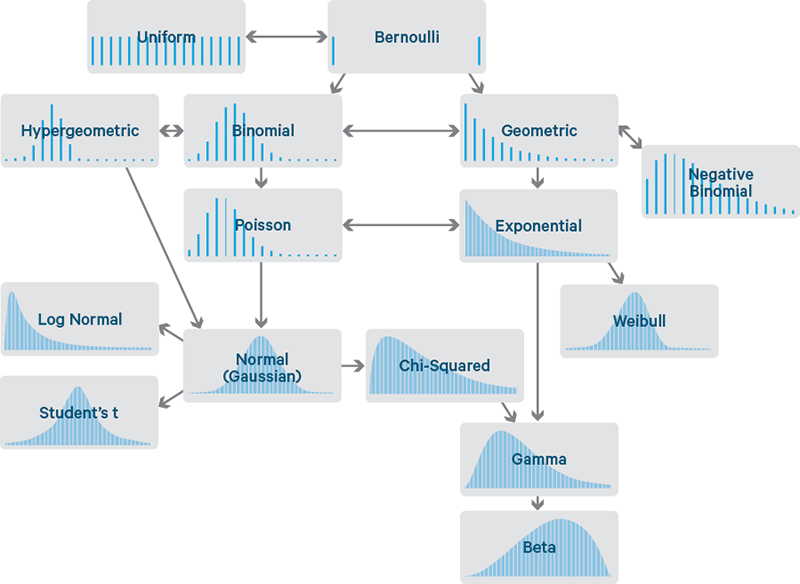
Probability distributions
- Given below are commonly found discrete and continuous probability distribution functions and their relationships with each other. Image credit and for a clear and simple explanation, check this article
- This is another interesting article showing all probability distributions, their equations and their relationships.
We can use the r() function to generate the random variates for these distributions. Below code generates some of these distributions and plots them using ggplot().
set.seed(1234)
normal<- rnorm(1000,mean=100,2)
tdist <- rt(n=1000,df = 50)
fdist <- rf(n=1000,df1 = 5, df2 = 100)
chisq <- rchisq(n=1000,df = 5)
exp <- rexp(n=1000,rate = 1)
pois <- rpois(n=1000,lambda = 5)
unif <- runif(n=1000,min = 5, max = 10)
geom <- rgeom(n=1000,prob= 0.5)
data <- cbind(normal,tdist,fdist,chisq,exp,pois,unif,geom)

transposed_df <-gather(as.data.frame(data),key="Name",value="Value")
transposed_df %>%
  ggplot() +
  geom_histogram(aes(x=Value,fill=Name),binwidth = 0.1) +
  labs(x=""
       ,y=""
       ,title = "Some Probability distribution functions"
       ,caption = varPlotCaption) +
  facet_wrap(~Name, scales = "free", nrow = 4) +
  theme_darklightmix(color_theme = ggplot_color_theme
                     ,legend_position = "none") +
  scale_fill_brewer(palette = "Set3")
#Plot the curves [ TO DO ]
#
# ggplot(transposed_df) +
#   stat_function(fun=to_be_done
#                 ,aes(x=Value)
#                 ,args = list(mean = mean(transposed_df$Value)
#                              ,sd = sd(transposed_df$Value))) +
#   facet_wrap(~Name, scales = "free", nrow = 3)
r,d,q and p functions in R
- r() : In the previous section, we saw the
r()function that we can use to generate random numbers satisfying different probability distributions. - q() : The q function is used to find the critical values from the probability distribution function. See Example 1 below in the Critical Values section
- p() : The p() is used to calculate the p-value from the probability distribution function. See Example 3 below in the Critical Values section
- d() : We can use the density function d() to find the height of the probability distribution at any given value
- More in this article
set.seed(1234)
dnorm(102,mean = mean(normal),sd = sd(normal))
## [1] 0.1177504normal<- rnorm(1000,mean=100,sd=2)
ggplot() +
stat_function(fun=dnorm
,aes(x=normal)
,args = list(mean = mean(normal)
,sd = sd(normal))) +
labs(x=""
,y=""
,subtitle="Normal distribution height"
,caption = varPlotCaption) +
theme_darklightmix(color_theme = ggplot_color_theme
,legend_position = "none") +
scale_fill_brewer(palette = "Set3")## Warning: `mapping` is not used by stat_function()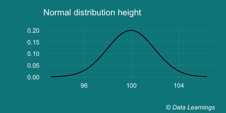
Hypothesis Testing & Null hypothesis
As per wikipedia, a null hypothesis is a default statement that there is no relationship between two events or no association among groups and that they are completely independent. And the central tasks of a statistician is to reject the null hypothesis and prove that the relationship exists. The opposite of null hypothesis is alternative hypothesis.
- Normally, we would either would either Reject the Null Hypothesis or Fail to reject the hypothesis. But there are couple of other possibilities and these are the Type I and Type II Errors
- Type I - False Positive : Error occur when we Reject the Null Hypothesis when actually we should not have rejected it
- Type II - False Negative : Error occur when we Fail to reject the Null hypothesis when we actually should have rejected it
The Type I error is actually the level of significance or the alpha level that we set. So if we set it at 0.05 it means the decision to reject the hypothesis when we should not have rejected it would happen 5% of the time. Hence, the Type I error is depends on what we set the alpha level. For example n certain medical studies the alpha is set at 0.001 if it involves harm to patients.
z-test, t-tests, chi-square test, ANOVA are examples of the types of statistical tests. Each of these tests have their own probability distribution and their own scores for testing the hypothesis.
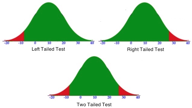
Two-tailed vs One-Tailed Hypothesis
- In the two-tailed hypothesis, we will reject the hypothesis if the sample mean falls in either tail of the distribution. The critical regions are shown below. Together the sum of their probability is 0.05.
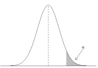
- One-tailed hypothesis is used when we are interested in the direction of the results. For example to test whether mean of one sample is greater than a given number. We will have only one critical region as shown below.
- When the alternative hypothesis is that the sample mean is greater, the critical region is on the right side of the distribution.
- When the alternative hypothesis is that the sample is smaller, the critical region is on the left side of the distribution.
Critical Values
Critical values are the values that indicate the edge of the critical region. Critical regions describe the entire area of values that indicate you reject the null hypothesis.
Any value observed in the Red Region indicates that the Null hypothesis should be rejected
Example 1
- In R, we can use the q() function to find the critical values.
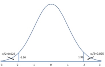
- So for a two-tailed test with 95% confidence interval in R we get the critical value as -1.96 for the left tail and +1.96 for the right tail and the region as shown in the picture.
- Since this is a two tailed test with alpha of 0.05, half of the alpha will be in the left tail and half in the right tail, hence p=0.025 is given in the below R code.
- Note : A normal distribution with a mean of 0 and a standard deviation of 1 is called a standard normal distribution.
qnorm(p=0.025,mean=0,sd=1,lower.tail = TRUE)## [1] -1.959964qnorm(p=0.025,mean=0,sd=1,lower.tail = FALSE)## [1] 1.959964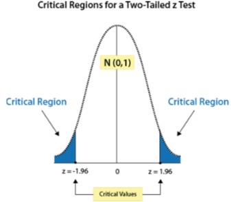
Example 2
- For a left tailed test with alpha = 0.01 we get the critical value as -2.33 and for a right tailed test this would be 2.33
qnorm(p=0.01,mean=0,sd=1,lower.tail = TRUE)## [1] -2.326348qnorm(p=0.01,mean=0,sd=1,lower.tail = FALSE)## [1] 2.326348Example 3
Find alpha for a given critical value Z = 1.96 for a right tailed test
pnorm(q=1.76,mean=0,sd=1,lower.tail = TRUE)## [1] 0.9607961P-value
- Assuming that the null hypothesis is true, the p-value gives the probability that the results from your sample data occurred by chance
- So, a low value indicates :
- Low probability that the results occurred by chance and
- that some relationship exists and
- that the results are statistically significant and
- hence the null hypothesis can be rejected
- For example, a p-value of .01 means there is only a 1% probability that the results from an experiment happened by chance
- A small p-value (typically ≤ 0.05) indicates strong evidence against the null hypothesis, so you reject the null hypothesis. A large p-value (> 0.05) indicates weak evidence against the null hypothesis, so you fail to reject the null hypothesis
- The p-value is derived based on the probability distribution of the test-statistic (eg t-score or chi-score) that its associated with. This is done using table which looks something like this
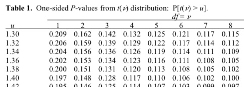
- Where \(\mu\) is test statistic (in this case the t-value) and \(df\) is the degrees of freedom. As you can see as the value of \(\mu\) increases, the probability or the p-value decreases. Example 3 above shows how we can find the p-value in R
Statistical tests
- Statistical tests are used for making inferences about data. They tell us whether an observed pattern is due to random chance or not.
- They are broadly classified :
- Parametric tests are used when the data is normally distributed
- Non-parametric when data is non-normal
- Commonly used Parametric tests
- Pearson correlation : Tests for the strength of association between continuous variables
- Spearman correlation is used when one or both of the variables are not assumed to be normally distributed and interval (but are assumed to be ordinal). The values of the variables are converted in ranks and then correlated.
- T-test : Look for the difference between the means of variables
- ANOVA : Tests the difference between group means after any other variance in the outcome variable is accounted for
- Regression : Assess if change in one variable predicts change in another variable
- Commonly used non-parametric tests
- Chi-square : Tests for the strength of association between categorical variables. The test compares actual results to the expected results.
- Wilcoxon rank-sum test
- Kruskal Wallis test
- T-test vs ANONA vs MANOVA
- T-tests are used when there is one independent variable (with 2 levels) and one dependent variable
- One-way ANOVA is used when there is one independent variable (with more than 2 levels) and one dependent variable
- Two-way ANOVA is used when there are more one independent variable (with more than 2 levels each) and one dependent variable
- MANOVA : Complicated and are used when there are more than one dependent variables
- In the next post, we will take a look at T-tests
Summary
- Type I - False Positive
- Type II - False Negative
- z-test, t-tests, chi-square test, ANOVA are examples of the types of statistical tests. Each of these tests have their own probability distribution and their own scores for testing the hypothesis.
- Assuming that the null hypothesis is true, the p-value gives the probability that the results from your sample data occurred by chance