Correlation

Correlation is a statistical technique that can be used to show how strongly two variables are linearly related to each other. The scatter plot shows that there is a inverse relationship, viz as wt increases mpg decreases.

mtcars %>%
  ggplot(aes(x=wt,y=mpg)) +
  geom_point()+
  geom_smooth(method="lm",se=F) +
  labs(subtitle="wt vs mpg"
  ,caption = varPlotCaption) +
  theme_darklightmix(color_theme = ggplot_color_theme) +
  scale_color_brewer(palette = "Set3")

## `geom_smooth()` using formula 'y ~ x'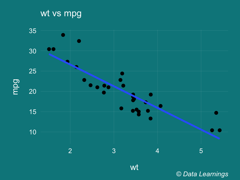

The Pearsons correlation coefficient using the cor() for mpg and wt is r = -0.867. Negative indicates inverse relationship. If we square r, we get the coefficient of determination or the proportion of variance accounted for.

cor(mtcars$mpg,mtcars$wt)

## [1] -0.8676594

cor(mtcars$mpg,mtcars$wt) ^ 2

## [1] 0.7528328

Now, how do we know whether the r is statistically significant ? We can use the t-test to establish if the correlation coefficient is significantly different from zero, and, hence that there is evidence of an association between the two variables. We will see this in more details in the regression section.

To do this, we can modify the t statistic formula,

\(t = \frac{\bar{x} - 0}{\sqrt{S^2 / n}}\)

as below

\(t = \frac{r - 0}{\sqrt{(1-r)^2 / (n-2)}}\)

We use the cor.test() from base R stats package. We get a t-value of -9.6 which is less than our critical value of -2.04, so it falls in the critical red region. Hence, we can reject the null hypothesis that states no relationship exists between mpg and wt.

cor.test(mtcars$mpg,mtcars$wt)

## 
##  Pearson's product-moment correlation
## 
## data:  mtcars$mpg and mtcars$wt
## t = -9.559, df = 30, p-value = 1.294e-10
## alternative hypothesis: true correlation is not equal to 0
## 95 percent confidence interval:
##  -0.9338264 -0.7440872
## sample estimates:
##        cor 
## -0.8676594

qt(p = 0.025,df=30)

## [1] -2.042272

• There are types of correlation
  • Pearson coefficient checks for linear relations
  • Spearman coefficient checks for rank or ordered relations, and
  • Kendall coefficient checks for degree of voting agreement.
• Each of these coefficients performs a progressively more drastic transform than the one before and has well-known direct significance tests (see help(cor.test)).

Simple Linear Regression

Simple Linear Regression is a linear function of one independent variable (say x) that can predict as accurately as possible the value of dependent variable (y). In simple notation we can understand this with a straight line equation y = mx + c, where m is the slope of the line and c is constant (value of y when x is 0).

We will use the lm() in base R to create our simple regression model and then use the summary() to investigate the model. We will look at each in details in the subsequent sections. But for now, lets see how some of these values are matching our correlation results.

We can see that r squared of 0.75 matches what we found in cor and the t statistic of the wt coefficient also matches what we found in cor.test. And this matches because just like correlation, the simple linear regression predicts the relationship between 2 variables.

Our model tells us that for every 1 unit change in wt, the mpg changes by the coeff estimate of wt which is -5.3445. In other words, the mpg is predicted to drop by -5.3445 units for every unit change in wt. It is predicted to be 37.2851 (the intercept) when the wt is 0

summary(lm(mpg~wt,data=mtcars))

## 
## Call:
## lm(formula = mpg ~ wt, data = mtcars)
## 
## Residuals:
##     Min      1Q  Median      3Q     Max 
## -4.5432 -2.3647 -0.1252  1.4096  6.8727 
## 
## Coefficients:
##             Estimate Std. Error t value Pr(>|t|)    
## (Intercept)  37.2851     1.8776  19.858  < 2e-16 ***
## wt           -5.3445     0.5591  -9.559 1.29e-10 ***
## ---
## Signif. codes:  0 '***' 0.001 '**' 0.01 '*' 0.05 '.' 0.1 ' ' 1
## 
## Residual standard error: 3.046 on 30 degrees of freedom
## Multiple R-squared:  0.7528, Adjusted R-squared:  0.7446 
## F-statistic: 91.38 on 1 and 30 DF,  p-value: 1.294e-10

Now lets understand the other values returned by our model

Residuals

The residuals are the difference between the dependent variable (y) and its values predicted by the linear model \(\widehat {y}\) . In our plot below, on the x-axis we have the wt variable. The dots represent the actual values of mpg and the + denotes the predicted value. The blue line is the regression line and the red line represents the residuals.

predicted  <- predict(lm(mpg~wt,data=mtcars))

mtcars %>%
ggplot(aes(x=wt,y=mpg)) +
geom_point() +
geom_point(aes(y=predicted), shape = 3) +
geom_smooth(method = "lm", se = FALSE, color = "blue", size = 0.2) +
geom_segment(aes(xend=wt,yend=predicted), color = "red", size = 0.3) +
labs (x = "wt"
      ,y = "Actuals (dots) and Predicted (+) mpg values"
      ,subtitle="wt vs mpg"
      ,caption = varPlotCaption) +
  theme_darklightmix(color_theme = ggplot_color_theme) +
  scale_color_brewer(palette = "Set3")

## `geom_smooth()` using formula 'y ~ x'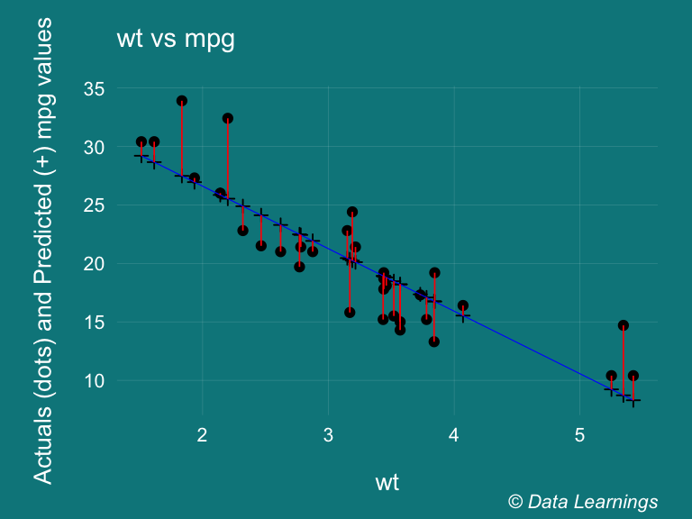

The residuals section of our model gives us a quick distribution of our residuals. It should be roughly symmetrical about mean, the median should be close to 0, the 1Q and 3Q values should ideally be roughly similar values.

t-value and p-values

We can use inferential statistics to completely explain our model.

The t statistic is the coefficient divided by the standard error. The SE being the standard deviation of the coefficient. The larger the t-value implies the coefficient is further away from 0 which implies that some relationship exists between dependent y and independent x.

Now, is this relationship statistically significant or its so just by some random chance. To determine that we can compare this t-value with the values in a Student t-distribution (which is a random distribution). The t-distribution gives us the p-value which is the probability that the t-value is due to some random chance. So, if the p-value is low means that probability of the t-value due to random chance is low and that the variable is a statistically significant

In regression, we are trying to discover whether the coefficients of our independent variables are really different from 0 (so the independent variables are having a genuine effect on your dependent variable) or if alternatively any apparent differences from 0 are just due to random chance. The null (default) hypothesis is always that each independent variable is having absolutely no effect (has a coefficient of 0) and you are looking for a reason to reject this theory.

R-squared

R squared gives us the proportion of the variance in the dependent variable that can be explained (or predicted) by the independent variable(s). The higher the better, in our case we can say that our can explain 75% of the variance in mpg.

If we look at the residuals plot above, we can see that the actual values are not far off from the predicted values. And the model can explain 75% of the that variance. If the predicted values were same as the actual values then we would have got a 100% R squared.

The R-squared gives us the overall feel for the model but the important thing is actually the P value that tells us how confident we can be that each individual variable has some correlation with the dependent variable. And we also have to look at the residual plots to look for any trends or patterns in them.

F-statistic

The F-Statistic gives us the overall significance our our model.

Any regression model has 3 errors :

Total Error = \(\sum {(y - \overline {y})^2}\)

Model Error = \(\sum {(\widehat {y} - \overline {y})^2}\)

Residual Error = \(\sum {(y - \widehat {y})^2}\)

• If we put this in a ANOVA table we get the F statistic. The F is the ratio of two variances (SSR/SSE) ie
  • The variance explained by the parameters in the model (sum of squares of regression, SSR) and t
  • The residual or unexplained variance (sum of squares of error, SSE).

It tells us if the error we saved by knowing the relationship between the independent variable and the dependent variable is more than the ‘left over’ or residual error then we have a significant overall model.

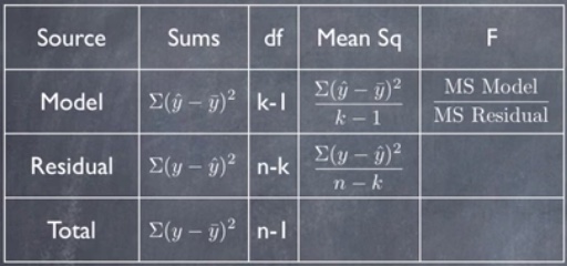
The Mean Sq column contains the two variances and 847.73/9.28 gives the F statistic i.e 91.375 for critical value of 4.17 (p=0.05)

anova(lm(mpg~wt,data=mtcars))

## Analysis of Variance Table
## 
## Response: mpg
##           Df Sum Sq Mean Sq F value    Pr(>F)    
## wt         1 847.73  847.73  91.375 1.294e-10 ***
## Residuals 30 278.32    9.28                      
## ---
## Signif. codes:  0 '***' 0.001 '**' 0.01 '*' 0.05 '.' 0.1 ' ' 1

qf(p=0.05, df1 = 1, df2 = 30, lower.tail = FALSE)

## [1] 4.170877

While R-squared provides an estimate of the strength of the relationship between your model and the response variable, it does not provide a formal hypothesis test for this relationship. The overall F-test determines whether this relationship is statistically significant. If the P value for the overall F-test is less than your significance level, you can conclude that the R-squared value is significantly different from zero.

Standardised Beta Coefficient

In regression, variables have different units and different scales of measurement. Eg unit of mpg is miles per gallon, whereas that of wt is lbs. The standardised coeff allows us to compare the their relative importance free of their units and scales. They have Standard Deviation as their units, so we can say every 1 SD change in wt the mpg will change by -0.867 SDs

Betas are calculated by subtracting the mean from the variable and dividing by its standard deviation. This results in standardized variables having a mean of zero and a standard deviation of 1. The higher the absolute value of the beta coefficient, the stronger the effect. It will always osciallate between 0 and 1.

Note that in our case it same as the Pearson Coefficient r value.

lm.fit <- lm(mpg~wt, data = mtcars)
QuantPsyc::lm.beta(lm.fit)

##         wt 
## -0.8676594

Confidence Intervals of the estimates

We can also find the CI of the estimate and its important to note that when the confint doesnt capture 0 then we have significant reationship.

confint(lm.fit)

##                 2.5 %    97.5 %
## (Intercept) 33.450500 41.119753
## wt          -6.486308 -4.202635

Summary

In this post we looked at few basic concepts of Linear Regression, mostly around the output given by the summary function. We saw the similarities between Correlation and Simple Linear Regression and how their how R squared and p-values match. We plotted the actual and predicted values and understood the concept of residuals. We also introducted the QuantPsyc package to find the standarised beta coefficients. In next article we will look at Multiple Linear Regression.